Model improvements Améliorations du modèle モデル改良
(Japanese translation needed!) (Japanese translation needed!)Date :Date : 日付 : August 28, 2020 28 août 2020 2020年8月28日
Author Auteur 著者 : Pascal Naidon
Disclaimer: I am a physicist, not an epidemiologist. Any comment from experts is welcome. Avertissement : Je suis physicien, pas épidémiologiste. Tout commentaire d'experts est le bienvenu. 免責事項:私は物理学者であり、疫学者ではありません。専門家からのコメントは大歓迎です。
Taking into account the age distribution
Originally, the renewal equation I have been using does not make a distinction between individuals of different ages. It was assumed that the population of infected individuals had a stable age distribution and likelyhood of developing severe form of the covid-19 or dying. The new surge of cases in Japan since June shows that the age distribution is very different: the majority of confirmed cases are young people, much less likely to become ill or die. For this reason, it is necessary to take the age of infectees into account. To do this, I generalised the renewal equation for the total number of newly infected individuals \(i(t)\), \[ i(t) =\beta(t)\Bigg(1 -\frac{1}{N}\int_{t_0}^{t}i(t_1)dt_1\Bigg)\int_{t_0}^{t}i(t_1)P(t-t_1)dt_1\label{renewalEq} \] to a set of coupled renewal equations for different age groups \(j\), \[ i_j(t) =\beta_j(t)\Bigg(1 -\frac{1}{N_j}\int_{t_0}^{t}i_j(t_1)dt_1\Bigg)\sum_{k}f_{j,k}\int_{t_0}^{t}i_k(t_1)P(t-t_1)dt_1\label{renewalEq2} \] The \(n=9\) different age groups are taken to be on 10-year intervals: {0-9, 10-19, 20-29, ... , 70-79, 80+} years old. The factor \(\beta_j\) represents the overall infection rate coefficient for the age group \(j\) and the fraction \(f_{j,k}\) represents the contribution to this infection rate by age group \(k\). Without in-depth information on social relations between different age groups, it is difficult to guess the values of these fractions. Nevertheless, one can consider two extreme limits and an ad-hoc intermediate situation:
- Different age groups do not interact: \(f_{j,k}\ = \delta_{i,j}\) (Kronecker delta)
- All age groups fully interact: \(f_{j,k} = 1/n\)
- Ad-hoc partial interaction: \(f_{j,k} \propto \exp(-(j-k)^2/d^2) \)
Guessing the real number of infections
Originally, I had assumed that the confirmed cases represented a fixed fraction \(p\) of the real number of infected individuals, which was guessed by assuming a certain infection fatality ratio (of about 1%). But the more active testing in Japan since May means most probably that higher fractions \(p\) have been tested over time.
An alternative assumption is to consider the case fatality ratio by age \(\text{CFR}_j\), i.e. the fraction of individuals expected to die among the confirmed cases \(c_j\) of age group \(j\). The total number \(d\) of cases expected to die is therefore \(d = \sum_j c_j \times\text{CFR}_j\). We can thus calculate the total case fatality ratio \( \text{CFR} = d / \sum_j c_j \). If the age distribution \(c_j\) of confirmed cases varies over time (which is the case since May), then so will the total case fatality ratio \(\text{CFR}\). However, we can assume that the total infection fatality ratio \(IFR\) (which is the ratio of deaths over the real number of infected) is constant. Under this assumption, we can calculate the changing fraction \(p\) of confirmed cases among the real number of infected individuals such that the \( \text{IFR} / p \) gives the case fatality ratio \(\text{CFR}\).
None of these two assumptions, either constant testing fraction \(p\) or constant IFR, are satisfactory. Nevertheless, to get an idea of the real number of infections, I have made calculations for each of these assumptions and used the lowest and highest results as lower and upper bounds.
As for the values of the case fatality ratios, I have used the values obtained on July 1st, at the end of the first wave in Japan: \[ \{\text{CFR}_j\} = \{ 0/306, 0/469, 1/3400, 4/2899, 14/2816, 33/2910, 99/1982, 266/1800, \ 552/1884 \} \label{CFRJapan} \] (source of the data: Toyo Keizai Online).
Readjusting the case fatality ratios
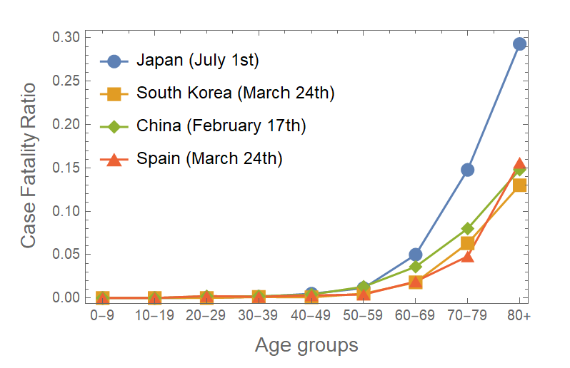
Figure 1 case fatality ratios for different countries. (sources: Toyo Keizai Online and ourworldindata.org)
Although the above case fatality ratios reproduce well the first wave of deaths (by construction), they overestimate the deaths which are starting to result from the current second wave. This overestimate occurs even though the use of age-dependent case fatality ratios takes into account the fact that many younger individuals unlikely to die have been confirmed with respect to the first wave. It is assumed that due to the lower number of tests during the first wave, fewer mild or asymptomatic cases were confirmed during the first wave, and the case fatality ratios were higher than they are now. In fact, it can be checked that the above case fatality ratios \eqref{CFRJapan} are typically twice larger (see figure 1) than those found in other countries like South Korea, where more active testing was done from the start. According to ourworldindata.org (data from the KCDC), the case fatality ratios in South Korea on March 24th were: \[ \{\text{CFR}_j\} = \{ 0, 0, 0, 0.11, 0.08, 0.5, 1.8, 6.3, 13 \}\% \label{CFRSKorea} \] To obtain more quantitative projections, I now assume that the case fatality ratios in Japan after 2020, June 21 are given by 80% of the South Korean case fatality ratios \eqref{CFRSKorea}. This gives much better agreement with the recently reported deaths.
AcknowledgmentsRemerciements謝辞
I am grateful to my colleagues at RIKEN, in particular at iTHEMS, for helpful discussions. Je remercie mes collègues de RIKEN, en particulier d'iTHEMS, pour leur aide. 理研の同僚、特にiTHEMSでの有益な議論に感謝します。

 riken.jp