Date :Date : 日付 :
May 13, 2020
13 mai 2020
2020年5月13日
Updated :Mise à jour : 更新 :
June 8, 2020
8 juin 2020
2020年6月08日
Author
Auteur
著者
:
Pascal Naidon
Disclaimer: The following shows an application of a simple and standard mathematical model of epidemic to the current new coronavirus SARS-CoV-2. The purpose is not to make accurate predictions but to show projections based on different simplifying assumptions and give a sense of typical orders of magnitude to be expected. I am a physicist, not an epidemiologist. I have made these calculations for my own understanding of the situation, as well as part of voluntary scientific support for the Saitama prefecture. These calculations have not been published in a peer-reviewed journal, and any comment from experts is welcome.
Avertissement : Ce qui suit montre une application d'un modèle mathématique simple et standard d'épidémie au nouveau coronavirus SARS-CoV-2 actuel. Le but n'est pas de faire des prévisions précises mais de montrer des projections basées sur différentes hypothèses simplificatrices et de donner une idée des ordres de grandeur typiques à prévoir. Je suis physicien, pas épidémiologiste. J'ai fait ces calculs à la fois pour ma propre compréhension de la situation, et en tant que soutien scientifique pour la région de Saitama. Ces calculs n'ont pas fait l'objet de publication dans une revue scientifique à comité de lecture. Tout commentaire d'experts est le bienvenu.
免責事項:以下で、現在の新型コロナウイルスSARS-CoV-2感染症の、単純かつ標準的な数学的モデルの適用を提示します。目的は、正確な予測を行うことではなく、さまざまな簡略化の仮定に基づいて予測を提示し、期待される感染規模を把握することです。 私は物理学者であり、疫学者ではありません。 これらの計算は、自分で状況を理解するため、そして埼玉県への自発的な科学的支援の一環として、行なったものです。学術誌に発表された査読付き研究ではありません。専門家からのコメントは大歓迎です。
A standard approach to model epidemics is the renewal equation. In such a model, one considers a population of \(N\) individuals and denotes by \(i(t)\) the instantaneous (daily) number of newly infected individuals at time \(t\), such that the total number of individuals who have been infected is,
Une approche standard de modélisation d'épidémie est l'équation de renouvellement. Dans un tel modèle, on considère une population d'individus \(N\) et on note \(i (t)\) le nombre instantané (quotidien) d'individus nouvellement infectés au temps \(t\), tel que le nombre total des personnes infectées est,
感染症の流行をモデル化する標準的なアプローチは、再生方程式です。このモデルでは、人口 \(N\) の集団を考え、時刻 \(t\) に新しく感染した個体の、即時的な(ここでは一日あたりの)数を \(i(t)\) で表します。時刻\(t\)においてすでに感染している個体の数 \(T(t)\) は、次式で与えられます:
\[
T(t) = \int_{t_0}^t i(t_1)dt_1\label{infected}
\]
where \(t_0\) denotes the starting time of the epidemic. The number of individuals who have not yet been infected (the susceptible individuals) is therefore:
où \(t_0\) indique l'instant du début de l'épidémie. Le nombre d'individus non encore infectés (les individus susceptibles) est donc:
ここで、\(t_0\) は感染の始まった時刻を表わします。したがって、まだ感染していない個体(感受性のある個体)の数は次のとおりです。
\[
S(t) = N - T(t)\label{susceptible}
\]
Here, it is assumed that individuals can be infected only once (i.e. there is long-term immunity, which is under debate for SARS-CoV-2).
Ici, il est supposé que les individus ne peuvent être infectés qu'une seule fois (c'est-à-dire qu'il existe une immunité à long terme, ce qui fait l'objet d'un débat pour le SRAS-CoV-2).
ここで、どの個体も同じ感染症には一度しか感染しないと想定されています(つまり長期的な免疫があるという仮定ですが、SARS-CoV-2についてそれが当てはまるかどうかには、議論の余地があります)。
Among the infected individuals, a certain number is infectious (that is to say, contagious to the not-yet-infected individuals). The number \(I(t)\) of infectious individuals is given by:
Parmi les individus infectés, un certain nombre est infectieux (c'est-à-dire contagieux aux individus non encore infectés). Le nombre \(I(t)\) d'individus infectieux est donné par:
感染個体のうち、一部の個体には感染力があります(つまり、感受性のある個体への伝染性です)。 感染者の個体数 \(I(t)\) は、
\[
I(t) =\int_{t_0}^{t} i(t_1) P(t - t_1) dt_1\label{infectious}
\]
where \(P(\tau)\) is the probability for an infected individual to be infectious after some time \(\tau\) since their infection.
Finally, the number of individuals newly infected by these infectious individuals is assumed to be proportional to both the number of infectious individuals \(I(t)\) and the number of susceptible individuals \(S(t)\):
où \(P (\tau)\) est la probabilité pour un individu infecté d'être infectieux après un certain temps \(\tau\) depuis son infection.
Enfin, le nombre d'individus nouvellement infectés par ces individus infectieux est supposé être proportionnel à la fois au nombre d'individus infectieux \(I (t)\) et au nombre d'individus susceptibles \(S (t)\):
ここで、 \(P(\tau)\) は、感染者が感染してから時間 \(\tau\) だけ経過して初めて感染力をもつ確率です。
最後に、これらの感染力のある個体によって新たに感染した個体の数は、感染力のある個体の数 \(I(t)\) と感受性個体の数 \(S(t)\) の両方に比例すると仮定します。
\[
i(t) =\beta(t)\frac{S(t)}{N} I(t)\label{renewalEq0}
\]
where the infection rate coefficient \(\beta(t)\) is related to the infectivity of the virus and the strength of social interactions between infectious and susceptible individuals. Combining all the above equations gives a closed equation on \(i(t)\) called the renewal equation:
où le coefficient de taux d'infection \(\beta (t)\) est lié à l'infectiosité du virus et à l'intensité des interactions sociales entre les individus infectieux et susceptibles. La combinaison de toutes les équations ci-dessus donne une équation fermée sur \(i (t)\) appelée équation de renouvellement:
ここで、感染係数 \(\beta(t)\) は、ウイルス自体の感染力と、感染力のある個体・感受性個体間の、社会的な相互作用の強さと連関します。上記のすべての方程式を組み合わせると、再生方程式と呼ばれる \(i(t)\) の、閉じた方程式が得られます。
\[
i(t) =\beta(t)\Bigg(1 -\frac{1}{N}\int_{t_0}^{t}i(t_1)dt_1\Bigg)\int_{t_0}^{t}i(t_1)P(t-t_1)dt_1\label{renewalEq}
\]
This model is of course very simplistic. Births, deaths due to other causes than the virus, and flux from other countries are neglected. Most importantly, the model assumes a homogeneous population with the same social interactions everywhere. It nonetheless constitutes a good starting point to understand the dynamics of the epidemic.
Ce modèle est bien sûr très simpliste. Les naissances, les décès dus à d'autres causes que le virus, ainsi que les flux entre pays sont négligés. Plus important encore, le modèle suppose une population homogène avec les mêmes interactions sociales partout . Il constitue néanmoins un bon point de départ pour comprendre la dynamique de l'épidémie.
もちろん、このモデルは非常に単純化されています。出生、ウイルス以外の原因による死亡、および他国からの流入を無視しています。最も重要なのは、社会相互作用が空間的にどこでも同じように起こっているという均質的な集団を仮定していることです。それでもなお、このモデルは流行のダイナミクスを理解するための良い出発点になります。
Determining the newly infections \(i(t)\)
What is known in practice is the numbers of confirmed cases every day. To relate these numbers to the number of infections \(i(t)\), I make the following assumptions:
-
The confirmed cases represent only a fraction \(f_\text{case}\) of the number of newly infections, because testing resources are limited and a large proportion of infected individuals are asymptomatic (they may not even be aware they have been infected). The fraction should therefore depend on the place and on the date. In the following, a specific \(f_\text{case}\) is considered for each place/country and it is assumed to be constant in time.
-
The confirmation of cases occurs after some delay from their infection date, because it takes some time for symptoms of the disease to appear (incubation period \(\tau_\text{incubation}\)) and it takes some time \(\tau_\text{confirmation}\) for a patient with symptoms to be tested and confirmed. The distribution of incubation period is intrinsic to the disease and has already been estimated (Linton et al., Lauer et al.), with an average incubation period of about 5 days. On the other hand, the distribution of confirmation delays is specific to each place. In the case of Japan, a typical number is 8 days. In principle, one should convolve the number of new infections \(i(t)\) with these delay distributions to obtain the number of confirmed cases. In practice, simply shifting by the average delays seems to be a good approximation.
It is therefore assumed that the daily number of confirmed cases is given by::
Détermination des nouvelles infections \(i(t)\)
Ce qui est connu dans la pratique, c'est le nombre de cas confirmés chaque jour. Pour relier ces nombres au nombre d'infections \(i(t)\), je fais les hypothèses suivantes:
-
Les cas confirmés ne représentent qu'une fraction \(f_\text{case}\) du nombre de nouvelles infections, car d'une part les ressources de test sont limitées, et d'autre part une grande proportion d'individus infectés sont asymptomatiques (ils ne savent peut-être même pas qu'ils ont été infectés). La fraction devrait donc dépendre en principe du lieu et de la date. Dans ce qui suit, un \(f_\text{case}\) spécifique est considéré pour chaque lieu/pays et il est supposé être constant dans le temps .
-
La confirmation des cas se produit après un certain délai à partir de leur date d'infection, car il faut un certain temps pour que les symptômes de la maladie apparaissent (période d'incubation \(\tau_\text{incubation}\)) et il faut un certain temps supplémentaire \(\tau_\text{confirmation}\) pour qu'un patient présentant des symptômes soit testé puis confirmé positif. La distribution de la période d'incubation est intrinsèque à la maladie et a déjà été estimée (Linton et al., Lauer et al.), avec une période d'incubation moyenne d'environ 5 jours. En revanche, la répartition des délais de confirmation est spécifique à chaque lieu. Dans le cas du Japon, un nombre typique est de 8 jours. En principe, il faut convoluer le nombre de nouvelles infections \(i(t)\) avec ces distributions de retard pour obtenir le nombre de cas confirmés. En pratique, le simple décalage par les retards moyens semble être une bonne approximation.
Il est donc supposé que le nombre quotidien de cas confirmés est donné par: :
新規感染の特定\(i(t)\)
実際に知られているのは、毎日確認された症例数です。これらの数値を感染数 \(i(t)\) に関連付けるために、次のことを前提としています。
-
感染個体の大部分は無症候性(感染していることに気付いていない可能性がある)であり、テストリソースが限られているため、確認された症例は、新たな感染者数の実際の値ではなく、そのうちの限られた一部の割合 \(f_\text{case}\) にすぎません。したがって、この割合は場所と日付に依存するはずです。以下では、特定の \(f_\text{case}\) の値を場所/国ごとに考慮し、時間変化せず一定であると仮定します。
-
病気の症状が現れるまでには時間がかかるため(潜伏期間\(\tau_\text{incubation}\))、感染の日付から少し遅れた時間 \(\tau_\text{confirmation}\) 後に症例が確認・確定されます。潜伏期間の従う確率分布は感染症ごとに固有ですが、すでに平均潜伏期間は約5日であると推定されています(Linton et al. , Lauer et al.)。一方、感染確認までの遅延の分布は場所によって異なります。日本の場合、典型的な値は8日です。原則として、確認された症例数は、これらの遅延分布を使用して、新しい感染者数 \(i(t)\) のたたみ込みで得られます。実際には、単純に遅延の平均値によるシフトが良い近似値であるようです。
このことから、確認された症例の1日あたりの数は次のように与えられると仮定します::
\[
c(t) = f_\text{case}\times i(t -\tau_\text{incubation} -\tau_\text{confirmation})\label{cases}
\]
where \(\tau_\text{incubation}\) = 5 days, \(\tau_\text{confirmation}\) = 8 days, and \(f_\text{case}\) is yet unknown and will be related to the infection fatality ratio \(f_\text{death}\) (see below). Since the daily number of confirmed cases \(c(t)\) can have large weekly fluctuations, it is averaged over a moving window of 7 days to obtain a smoother curve. Then equation \eqref{cases} is inverted to obtain the daily number of infections \(i(t)\).
Determining the infectious individuals \(I(t)\)
To obtain the number of infectious individuals from\eqref{infectious}, one needs to know the probability \(P(\tau)\) for being infectious after some time \(\tau\) since infection. The probability \(P\) is assumed to be proportional to the serial time distribution, which is the distribution \(g(\tau)\) of times \(\tau\) between the illness onset of an infectee and the illness onset of their infector, i.e.
où \(\tau_\text{incubation}\) = 5 jours, \(\tau_\text{confirmation}\) = 8 jours et \(f_\text{case}\) est encore inconnu et sera lié au taux de mortalité par infection \(f_\text{death}\) (voir ci-dessous). Étant donné que le nombre quotidien de cas confirmés \(c(t)\) peut présenter de grandes fluctuations hebdomadaires, il est moyenné sur une fenêtre glissante de 7 jours pour obtenir une courbe plus lisse. Ensuite, l'équation \eqref{cases} est inversée pour obtenir le nombre quotidien d'infections\(i (t)\).
Détermination des individus infectieux \(I (t)\)
Pour obtenir le nombre d'individus infectieux à partir de \eqref{infectious}, il faut connaître la probabilité \(P (\tau)\) d'être infectieux après un certain temps \(\tau\) depuis l'infection. La probabilité \(P\) est supposée être proportionnelle à la distribution de temps de série , qui est la distribution \(g(\tau)\) des temps \(\tau\) entre le début de la maladie d'une personne infectée et l'apparition de la maladie de son infecteur,
ここで、\(\tau_\text{incubation}\)= 5日、\(\tau_\text{confirmation}\)= 8日ですが、 \(f_\text{case}\)はまだ不明かつ感染致死率\(f_\text{death}\)と関連しています(下記参照)。確認された症例の1日あたりの数 \(c(t)\) には週ごとに大きく変動する可能性があるため、より滑らかな曲線を得るために、7日間のデータにわたって平均化した値を用います。次に、方程式 \eqref{cases} を逆算し、日ごとの感染者数 \(i(t)\) を導出します。
感染者数 \(I(t)\) の特定
\eqref{infectious}から感染者の数を取得するには、感染後に時間が\(\tau\)だけ経ってから感染力を持つ確率 \(P(\tau)\) を知る必要があります。確率 \(P\) は、シリアル時間分布に比例すると見なされます。シリアル時間分布とは、感染者の発症時刻とその二次感染者の発症時刻の差 \(\tau\) の従う分布\(g(\tau)\)です:
\[
P(\tau) = \tau_\text{infectious} g(\tau)
\]
where the time \(\tau_\text{infectious}\) is the integral of \(P\) and corresponds to the average infectious period of an infected individual.
The serial time distribution of SARS-CoV-2 has been estimated (Nishiura et al.), and accordingly \(g(t)\) is assumed to be given by the log-normal distribution with parameters \(\mu = 1.386\) days and \(\sigma = 0.568\) days.
On the other hand, the average infectious period \(\tau_\text{infectious}\) is to my knowledege unknown. Since \(P\) is a probability, it cannot be larger than 1, which sets an upper limit of 4.85 days for \(\tau_\text{infectious}\). It is unreasonable to think that individuals are contagious for less than 1 day, so in the following I use 1 day and 4.85 days as the extreme values for the average infectious period. Note that in the following analyses, the choice of \(\tau_\text{infectious}\) affects the number of infectious individuals, which is important for the termination of the epidemic, but it does not affect the evolution of other quantities before the end of the epidemic.
Determining the reproduction number
The ratio of \( i(t)\) and \( I(t)/\tau_\text{infectious}\) gives the effective reproduction number
où le temps \(\tau_\text{infectious}\) est l'intégrale de \(P\) et correspond à la période infectieuse moyenne d'un individu infecté.
La distribution de temps de série du SARS-CoV-2 a été estimée (Nishiura et al.), et en conséquence \(g(t)\) est supposé être donné par la distribution log-normale avec les paramètres \(\mu = 1,386\) jours et \(\sigma = 0,568\) jours .
En revanche, la période infectieuse moyenne \(\tau_\text{infectious}\) est à ma connaissance inconnue. Puisque \(P\) est une probabilité, elle ne peut pas être supérieure à 1, ce qui fixe une limite supérieure de 4,85 jours pour \(\tau_\text{infectious}\). Il est déraisonnable de penser que les individus sont contagieux pendant moins d'un jour, donc dans la suite j'utiliserai 1 jour et 4,85 jours comme valeurs extrêmes pour la période infectieuse moyenne . Notez que dans les analyses suivantes, le choix de \(\tau_\text{infectious}\) affecte le nombre d'individus infectieux, ce qui est important pour la fin de l'épidémie, mais il n'affecte pas l'évolution des autres quantités avant la fin de l'épidémie.
Détermination du nombre de reproduction
Le rapport \(i (t)\) et \(I (t) / \tau_\text{infectious}\) donne le nombre de reproduction effectif
ここで、時間\(\tau_\text{infectious}\)は\(P\)の積分であり、感染した個人の平均感染期間に対応しています。
SARS-CoV-2のシリアル時間分布は、 Nishiura et al.にて推定されており、< em>それによると \(g(t)\) は、パラメータ\(\mu = 1.386\)日と\(\sigma = 0.568\)日で決まる log-normal distribution によって与えられると仮定されています。
一方、平均的な感染期間 \(\tau_\text{infectious}\) は、私の知る限りでは不明です。\(P\)は確率であるため、1以下です。これにより、 \(\tau_\text{infectious}\) の上限は4.85日と決まります。伝染性が1日未満であると考えるのは不合理です。そのため、以下では、平均感染期間の最小値・最大値として1日と4.85日を用います 。ただし以下の分析では、\(\tau_\text{infectious}\)の値の選び方が、感染者の数に影響を与えることに注意してください。これは、流行の終息に重要ですが、それ以前のその他の量の変化には影響しません。
再生数の決定
\(i(t)\)と\(I(t)/\tau_\text{infectious}\)の比率により、次式の有効再生数が決まります:
\[R_e(t) =\tau_\text{infectious}\beta(t)\frac{S(t)}{N}.\label{R_e}\]
From \eqref{infectious}, one can see that \( I(t)/\tau_\text{infectious} = \int_{t_0}^{t} i(t_1) g(t - t_1) dt_1\) is the average of the most recent daily infections over the serial time. The effective reproduction number \(R_e\) thus compares the new daily infections to this average of recent daily infections. If \(R_e > 1\) the daily infections increase, and if \(R_e < 1\) the daily infections decrease. The effective reproduction number therefore gives a measure of the epidemic trend.
One can see from \eqref{R_e} that a decrease in the effective reproduction number may be either due to a decrease in social interactions (through \(\beta(t)\) or a decrease in the number of susceptible individuals (herd immunity). To get an idea of the variations in social interactions, one can divide the effective reproduction number by \(S(t)/N\), giving the basic reproduction number,
A partir de \eqref{infectious}, on peut voir que \(I (t) / \tau_\text{infectious} = \int_{t_0} ^{t} i (t_1) g (t - t_1) dt_1\) est la moyenne des infections quotidiennes les plus récentes sur la période de temps de série. Le nombre de reproduction effectif \(R_e\) compare ainsi les nouvelles infections quotidiennes à cette moyenne des infections quotidiennes récentes. Si \(R_e > 1\) les infections quotidiennes augmentent et si \(R_e < 1\) les infections quotidiennes diminuent. Le nombre de reproduction effectif donne donc une mesure de la tendance épidémique.
On peut voir dans \eqref{R_e} qu'une diminution du nombre de reproduction effectif peut être due soit à une diminution des interactions sociales (à travers \(\beta (t)\)) soit à une diminution du nombre d'individus sensibles (immunité collective). Pour se faire une idée des variations des interactions sociales, on peut diviser le nombre de reproduction effectif par \(S (t) /N\), ce qui donne le nombre de reproduction de base ,
\eqref{infectious}から、\(I(t)/\tau_\text{infectious} =\int_{t_0} ^{t} i(t_1)g(t-t_1)dt_1\)が、シリアル時間における、最近日の感染者数の平均がわかります。したがって、有効再生算数\(R_e\)は、日毎の新規感染者数を、先程の、最近日の感染者数の平均と比較します。\(R_e > 1\)の場合、日毎の感染者数が増加し、\(R_e < 1\)の場合、減少します。 したがって、実効再生算数は、流行の傾向の指標となります。
\eqref{R_e}から、実効再生算数の減少は、社会的相互作用の減少 (\(\beta(t)\)による) または感受性個体の数の減少が原因である可能性があることがわかります(集団免疫)。社会的相互作用の変動について理解するために、実効再生算数を \(S(t)/N\) で割り、基本再生算数を得ます:
\[R_0(t) = \tau_\text{infectious}\beta(t)\label{R_0}\]
which is simply proportional to the infection rate coefficient \(\beta(t)\). Note that both reproduction numbers thus constructed from \(i(t)\) are independent of the assumed value for \(\tau_\text{infectious}\).
Determining the fatal cases
A certain fraction \(f_\text{case-death}\) of the confirmed cases eventually decease. This fraction is called the case fatality ratio. To find the number of deceased individuals, one needs to multiply the number of cases \(c(t)\) by this fraction \(f_\text{case-death}\) and convolve it with the cumulative distribution of time delays between confirmation and death. What is known from hospitals is the dsitribution \(P_D\) of delays between admission and death. Assuming that admission to hospital occurs after some time \(\tau_\text{admission}\) from confirmation, one obtains the number of deceased individuals:
qui est simplement proportionnel au coefficient de taux d'infection \(\beta (t)\). Notez que les deux nombres de reproduction ainsi construits à partir de \(i (t)\) sont indépendants de la valeur supposée pour \(\tau_\text{infectious}\).
Détermination des cas mortels
Une certaine fraction \(f_\text{case-death}\) des cas confirmés finit par disparaître. Cette fraction est appelée taux de létalité . Pour trouver le nombre de personnes décédées, il faut multiplier le nombre de cas \(c(t)\) par cette fraction \(f_\text{case-death}\) et le convoluer avec la fonction de répartition des délais entre confirmation et décès. Ce qui est connu des hôpitaux, c'est la distribution \(P_D\) de délais entre l'admission et le décès. En supposant que l'admission à l'hôpital a lieu après un certain temps \(\tau_\text{admission}\) à partir de la confirmation , on obtient le nombre de personnes décédées:
これは単純に感染係数 \(\beta(t)\) に比例します。このように \(i(t)\) から構成された再生算数はどちらも、 \(\tau_\text{infectious}\) の想定値によらないことに注意してください。
死亡症例の特定
確認症例の一部 \(f_\text{case-death}\) は最終的には亡くなります。この割合は、致死率と呼ばれます。死亡者数を求めるには、症例数 \(c(t)\) に、この割合 \(f_\text{case-death}\) を掛けて、確認から死亡に至るまでの時間遅延の累積分布を畳み込む必要があります。病院でわかるのは、入院から死亡までの遅延の分布 \(P_D\) です。 病院への入院が、発症を確認してから\(\tau_\text{admission}\) 後に行われると仮定すると、死亡者の数が求まります(訳者注:hospital admission は 入院のこと):
\[
D(t) = f_\text{case-death}\int_{0}^{t-\tau_\text{admission}-t_0} c(t-\tau_\text{admission}-\tau) P_D(\tau) d\tau
\]
For Japan, the distribution \(P_D\) is taken to be a Weibull distribution of parameters \(\alpha=1.361\) and \(\beta=12.96\), obtained by fitting data from Saitama hospitals. When the cumulated number of deaths has reached a plateau after an initial exponential growth, it is easy to adjust \(f_\text{case-death}\) to match the height of the plateau. The admission delay can then be adjusted to match the curve \(D(t)\) with the observed data and is found to be around 3 days.
Since the number of confirmed cases is itself a fraction \(f_\text{case}\) of all the infections (Eq.\eqref{cases}), one obtains the fraction \(f_\text{death} = f_\text{case} f_\text{case-death} \) of deceased individuals among infected individuals. This fraction is the infection fatality ratio (IFR). Unlike \(f_\text{case}\), which depends on the testing capacity and policy of each country, the infection fatality ratio \(f_\text{death} \) should have similar values across different countries (although it could depend on the hospital conditions and capacities, as well as health conditions and genetics of the populations). For this reason, once \(f_\text{case-death}\) has been determined, it is preferable to express \(f_\text{case}\) in terms of \(f_\text{death}\). As seen below, the IFR is estimated to be somewhere between 0.02% and 4%, likely around 1%.
Several studies have estimated the IFR: 0.64% (0.50-0.78%) [Meyerowitz-Katz et al], 1.04% (0.77%,1.38%) [Grewelle et al], and 0.26% (0.02%-0.86%) [Ioannidis].
Making projections
Once the above parameters have been fixed, it is possible to propagate the renewal equation \eqref{renewalEq} forward in time. For this purpose, one needs to specify the time dependence of the infection rate coefficient \(\beta(t)\), or equivalently the basic reproduction number \(R_0(t)\) defined in \eqref{R_0}. This is of course impossible, as one cannot predict the evolution of social interactions, so one can instead consider different plausible scenarios.
- The simplest scenario (scenario A) assumes that the basic reproduction number remains the same as it has been in the last few days (i.e. keeping current social restrictions), and from a certain date changes to a final value (return to normal life) over a certain transition period. This final value is set to the highest value (typically around 2) observed just before it was decreased by social distancing.
-
In a second scenario (scenario B), the return to normal life creates a second wave of infections. This new wave of infection is eventually detected, and new social restrictions are put in place from a certain date, over a transition period.
In the following, the transition periods are taken to be one month, which seems to be the typical transition time for past variations of \(R_0(t)\).
To describe more realistically the termination of the epidemic, the number of infectious individuals of \eqref{infectious} and the number of newly infected individuals of \eqref{renewalEq0} are rounded to the nearest integers. Finally, when the number of infectious individuals reaches zero, the epidemic is considered to be terminated.
Pour le Japon, on suppose que la distribution \(P_D\) est donnée par une distribution de Weibull avec les paramètres \(\alpha = 1.361 \) et \(\beta = 12.96 \), obtenue en faisant un ajustement sur les données des hôpitaux de Saitama. Lorsque le nombre cumulé de décès a atteint un plateau après une croissance exponentielle initiale, il est facile d'ajuster \(f_\text{case-death}\) pour correspondre à la hauteur du plateau. Le délai d'admission peut ensuite être ajusté pour faire correspondre la courbe \(D(t)\) avec les données observées, et est typiquement de 3 jours.
Le nombre de cas confirmés étant lui-même une fraction \(f_\text{case}\) de toutes les infections (Eq. \eqref{cases}), on obtient la fraction \(f_\text{death} = f_\text{case} f_\text{case-death}\) d'individus décédés parmi les individus infectés. Cette fraction est le taux de mortalité par infection (IFR). Contrairement à \(f_\text{case}\), qui dépend de la capacité de test et de la politique de chaque pays, le taux de mortalité par infection \(f_\text{death}\) devrait avoir des valeurs similaires dans différents pays (bien qu'il puisse dépendre des conditions et capacités hospitalières, ainsi que des conditions sanitaires et génétiques des populations). Pour cette raison, une fois \(f_\text{case-death}\) déterminé, il est préférable d'exprimer\(f_\text{case}\) en termes de \(f_\text{death}\). Comme indiqué ci-dessous, le taux de mortalité par infection est estimé entre 0,02% et 4%, probablement proche de 1%.
Plusieurs études ont fait des estimations de ce taux : 0.64% (0.50-0.78%) [Meyerowitz-Katz et al], 1.04% (0.77%,1.38%) [Grewelle et al], and 0.26% (0.02%-0.86%) [Ioannidis].
Projections
Une fois les paramètres ci-dessus fixés, il est possible de propager dans le temps l'équation de renouvellement \eqref{renewalEq}. À cette fin, il faut spécifier la dépendance temporelle du coefficient de taux d'infection \(\beta(t)\), ou de manière équivalente du nombre de reproduction de base \(R_0 (t)\) défini dans \eqref{R_0}. Ceci est bien sûr impossible, car on ne peut pas prédire l'évolution des interactions sociales. On peut donc plutôt envisager différents scénarios plausibles.
- Le scénario le plus simple (scénario A) suppose que le nombre de reproduction de base reste le même qu'au cours des derniers jours (c'est-à-dire en conservant les restrictions sociales actuelles) et, à partir d'une certaine date, passe à une valeur finale (retour à la vie normale) sur une certaine période de transition. Cette valeur finale est fixée à la valeur la plus élevée (généralement autour de 2) observée juste avant d'être diminuée par la distanciation sociale.
-
Dans un deuxième scénario (scénario B), le retour à la vie normale crée une deuxième vague d'infections. Cette nouvelle vague d'infections est finalement détectée, et de nouvelles restrictions sociales sont mises en place à partir d'une certaine date et ce progressivement sur une période de transition.
Dans ce qui suit, les périodes de transition sont considérées comme étant d'un mois, ce qui semble être le temps de transition typique pour les variations passées de \(R_0(t)\).
Pour décrire de manière plus réaliste la fin de l'épidémie, le nombre d'individus infectieux obtenu à partir de \eqref{infectious} et le nombre d'individus nouvellement infectés obtenu à partir de \eqref{renewalEq0} sont arrondis aux entiers les plus proches. Enfin, lorsque le nombre d'individus infectieux atteint zéro, l'épidémie est considérée comme terminée.
日本については、 \(P_D\) の分布は、埼玉県の病院からデータをフィッティングすることによって取得された、パラメーター \(\alpha = 1.361\) および \(\beta = 12.96 \) のワイブル分布と見なされます。
初期の指数関数的増加の後に累積死亡数が頭打ち(プラトー)に達した場合、プラトーの高さに合わせて \(f_\text{case-death}\) を調整するのは簡単です。次に、入院遅延を調整して(約3日間)、曲線 \(D(t)\) を観測データとフィッティングさせることができます。
確定症例者数は、それ自体がすべての感染者数の一部 \(f_\text{case}\) であるため(式\eqref{cases})、全感染者のうち、死亡した感染者の割合 \(f_\text{death} = f_\text{case}\(f_\text{case-death}\) が得られます。この割合が、感染致死率です。各国の検査キャパシティ・検査方針に依存する \(f_\text{case}\) とは異なり、感染致死率\(f_\text{death}\)は、異なる国で同様の値を持つ必要があります(ただし、病院の状態とキャパシティ、ならびに人口の健康状態と遺伝的要因には依存する可能性はあります)。このため、\(f_\text{case-death}\)が決定されたら、\(f_\text{case}\)を\(f_\text{death}\)で表すことが望ましいです。以下に見られるように、感染による死亡率は0.02%から4%の間のどこかと推定されています。
いくつかの研究はIFRを推定しました:0.64% (0.50-0.78%) [Meyerowitz-Katz et al], 1.04% (0.77%,1.38%) [Grewelle et al], and 0.26% (0.02%-0.86%) [Ioannidis].
定量的な見積もり
上記のパラメータをいったん固定すれば、再生方程式\eqref{renewalEq}を時間前向きに計算することができます。この目的のために、感染係数\(\beta(t)\)の時間依存性、あるいはまったく同じことですが\eqref{R_0}で定義された基本再生産数 \(R_0(t)\) を決定する必要があります。社会的相互作用の時間変化を予測することはできないため、これはもちろん不可能ですから、その代わりに、尤もらしいシナリオを考慮できます。
- 最も単純なシナリオ(シナリオA)では、基本再生産数が過去数日間と同じまま(つまり、現在の社会的な制限を維持する)だが特定の日からは特定の移行期間を経て、ある最終値に変化する(通常生活に戻る)ことを考えます。この最終値は、社会的距離によって減少する直前に観測された最高値(通常は約2)に設定されます。
-
2番目のシナリオ(シナリオB)では、通常の生活に戻ると、感染の2番目の波が発生します。この新しい感染の波が最終的に検出され、移行期間中に特定の日から新しい社会的制限が課されます。
以下では、その移行期間は1か月と見なされます。これは、\(R_0(t)\) の過去の変動の典型的な移行時間と思われます。
流行の終息をより現実的に説明するために、\eqref{infectious}の感染性個体の数と\eqref{renewalEq0}の新たに感染した個体の数を、最も近い整数に丸めこみます。最後に、感染者の数がゼロになると、流行は終息したと見なされます。
The SEIR model
Le modèle SEIR
SEIRモデル
The SEIR model is a very commonly used compartmental model to describe epidemics. It divides the population into four categories: susceptible (S), exposed (E), infectious (I) and removed (R), and the numbers of individuals in these four categories are assumed to follow a set of differential equations.
It can be shown [Inaba 2018][Champredon et al. 2018] that the SEIR model is particular case of the renewal equation model \eqref{renewalEq} corresponding to an infectious probability \(P\) resulting from the convolution of exponential distributions (or more generally Erlang distributions in the SEIR extensions).
Le modèle SEIR est un modèle compartimental très couramment utilisé pour décrire les épidémies. Il divise la population en quatre catégories: sensibles (S), exposées (E), infectieuses (I) et retirées (R), et le nombre d'individus dans ces quatre catégories est supposé suivre un ensemble d'équations différentielles.
On peut montrer [Inaba 2018][Champredon et al. 2018] que le modèle SEIR est un cas particulier du modèle d'équation de renouvellement \eqref{renewalEq} correspondant à une probabilité infectieuse \(P\) résultant de la convolution de distributions exponentielles (ou plus généralement de distributions d'Erlang dans les extensions de SEIR).
SEIRモデルは、流行を説明するために非常に一般的に使用されているコンパートメントモデルです。 人口を4つのカテゴリに分類します:感受性(S)、曝露(E)、感染性(I)、除去(R)。これらの4つのカテゴリの個人の数は、一連の微分方程式に従うと仮定されます。
SEIRモデルは、指数分布(またはより一般的にはSEIR拡張のアーラン分布)の畳み込みから生じる感染確率\(P\)に対応する再生方程式モデル\eqref{renewalEq}の特定のケースであることを示すことができます[Inaba 2018][Champredon et al. 2018]。
The reproduction number calculation from the Nishiura team
Le calcul du nombre de reproduction de l'équipe Nishiura
西浦チームの再生産数の計算
\[
i_\text{domestic}(t) = R_e(t) \int i_\text{total}(t-\tau) g(\tau) \frac{F(T-\tau)}{F(T-t+\tau)}
\]
which is a bit more sophisticated than \eqref{renewalEq}, as it makes a distinction between the domestic cases (who contracted the virus in Japan) and the total cases (who can have contracted the virus abroad), and in addition the cumulative distribution \(F\) of time delay from infection to reporting is used to account for cases that have not yet been reported but already infected. In the method presented here, I approximate the total cases as domestic cases, and I calculate the reproduction number only from reported cases, which limits the calculation to 13 days before now.
Moreover, the Nishiura team uses a more advanced techniques to obtain the number of newly infected individuals from the confirmed cases, using the dates of symptom onsets known for some cases. In my case, I simply scale and shift in time the confirmed cases to obtain an estimate of the newly infected individuals.
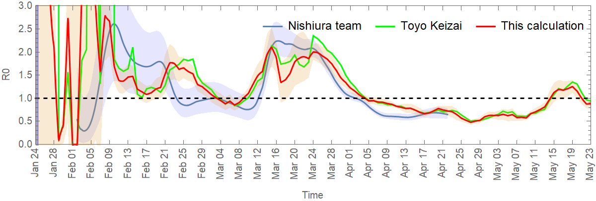
The method presented here is therefore a simplified version of the method used by the Nishiura team. The website Toyo Keizai also provides a simplified calculation of the effective reproduction number, based on the simple formula: (New cases in past 7 days / New cases in 7 days before that) ^ (mean generation time / length of reporting interval), where the mean generation time is taken to be 5 days, and length of reporting interval is supposed to be 7 days. When shifted in time by 13 days, this formula is in good agreement with my own calculation, as shown in the figure below for the reproduction number in Japan.
qui est un peu plus sophistiquée que \eqref{renewalEq}, car il y est fait une distinction entre les cas domestiques (qui ont contracté le virus au Japon) et le nombre total de cas (qui peuvent avoir contracté le virus à l'étranger), et de plus, la fonction de répartition \(F\) du délai entre l'infection et la confirmation est utilisée pour tenir compte des cas qui n'ont pas encore été signalés mais qui sont déjà infectés. Dans la méthode présentée ici, je considère le nombre total de cas comme des cas domestiques, et je calcule le nombre de reproduction uniquement à partir des cas signalés, ce qui limite le calcul à 13 jours auparavant.
De plus, l'équipe de Nishiura utilise des techniques plus avancées pour obtenir le nombre d'individus nouvellement infectés à partir des cas confirmés, en utilisant les dates d'apparition des symptômes connues pour certains cas. Dans mon cas, je multiplie et décale simplement dans le temps les cas confirmés pour obtenir une estimation des individus nouvellement infectés.
La méthode présentée ici est donc une version simplifiée de la méthode utilisée par l'équipe de Nishiura. Le site de Toyo Keizai fournit également un calcul simplifié du nombre de reproduction effectif, basé sur une formule simple: (Nouveaux cas dans les 7 derniers jours / Nouveaux dans les 7 jours encore avant) ^ (temps de génération moyen / délai de rapport), où le temps de génération moyen est fixé à 5 jours, et le délai de rapport est fixé à 7 jours. Lorsqu'elle est décalée dans le temps de 13 jours, cette formule est en bon accord avec mon propre calcul, comme le montre la figure ci-dessous pour le nombre de reproduction au Japon.
これは\eqref{renewalEq}よりも、やや洗練されています。国内の症例(日本でウイルスに感染したケース)と合計の症例(海外でウイルスに感染した可能性があるケースも含む)を区別し、さらに感染から報告までの時間遅延の累積分布 \(F\)を、まだ報告されていないがすでに感染している症例を記述するために用います。ここで紹介する方法では、全体の症例を国内の症例と近似し、報告された症例のみから再生算数を計算します。これにより、各日付から遡ること13日前の値の計算に制限されます。
さらに西浦チームは、いくつかの症例で知られている症状の発症日データを用いて、確定症例から新規感染者数を取得するために、より高度な手法を使用しています。私の計算では、確定症例を時間的にスケーリング・シフトさせ、新規感染者数の推定値を求めます。
そのため、ここで紹介する方法は、西浦チームが使用した方法を簡略化したものです。
東洋経済のウェブサイトでは、次の単純な式に基づいて、実効再生算数の簡単な計算を提供しています:「(直近7日間の新規陽性者数/その前7日間の新規陽性者数)^(平均世代時間/報告間隔)」。ここで平均世代時間は5日、報告間隔は7日と仮定します。13日間シフトを行なうと、この式は私の計算とよく一致します。下の図は、日本での再生算数を示しています。
France
France
フランス
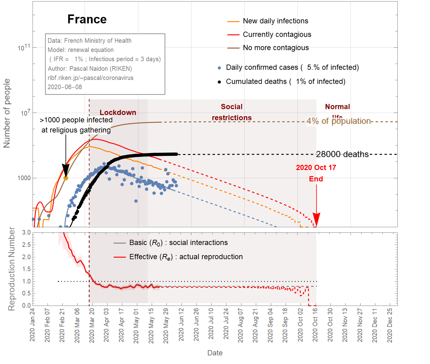
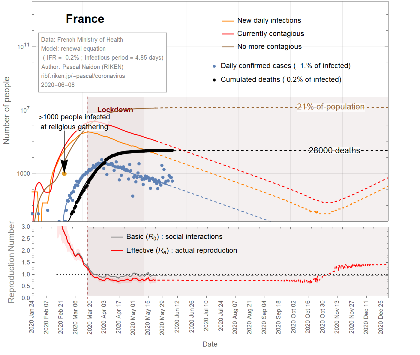
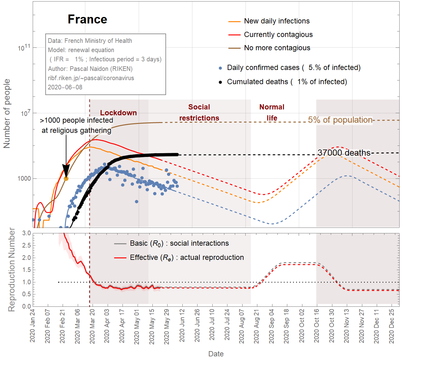
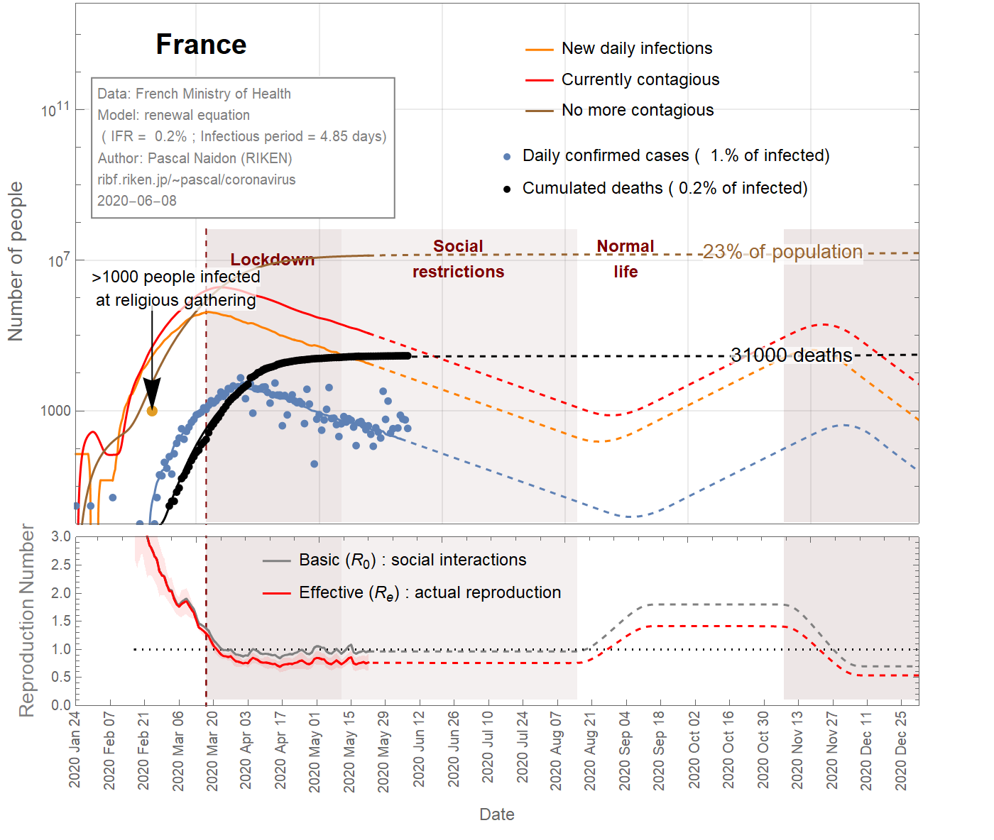
In the case of France, a large cluster of people was infected at a religious gathering involving 2500 people between February 17th and 24th, 2020. It is believed that at least 1000 people became infected [Ref], subsequently spreading the virus in different parts of the country as they went back home. Taking this minimum number of infections at the latest date (Feb 24th) sets a maximum value for the infection fatality ratio (IFR) of about 4% (see Fig 1). It could be much smaller as there could be many more people infected. However, the IFR cannot be smaller than 0.045%, otherwise the predicted number of infected individuals would exceed the total population. Even with an IFR of 0.2%, the number of infections is such that a significant fraction (>20%) of the population gets eventually infected (see Fig 3), and the decrease of observed cases after the lockdown would be due in great part to herd immunity, rather than the restriction of social interactions (the basic reproduction number would remain close to 1). This scenario does not seem very likely, and one can take 0.2% as a reasonable lower bound for the IFR.
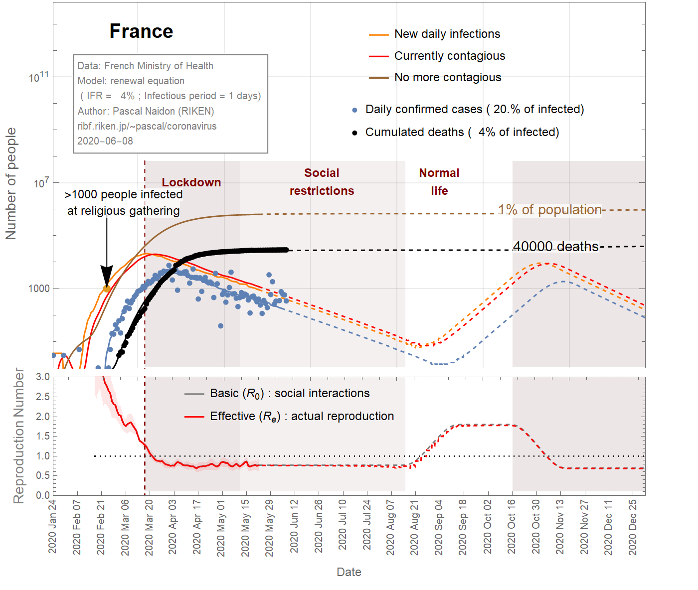
Thus one can conclude that the infection fatality ratio for France is somewhere between 4% and 0.2%. Figure 2 shows the results for an intermediate value of 1%. In this case, 4% of the French population has been infected.
Dans le cas de la France,
un grand groupe de personnes a été infecté lors d'un rassemblement religieux impliquant 2500 personnes entre le 17 et le 24 février, 2020 . On pense qu'au moins 1000 personnes ont été infectées [
Réf ], propageant ensuite le virus dans différentes parties du pays alors qu'elles rentraient chez elles. La prise en compte de ce nombre minimal d'infections à la dernière date du rassemblement (24 février) définit une valeur maximale pour le taux de mortalité par infection (IFR) d'environ 4% (voir la figure 1). Il pourrait être beaucoup plus petit car il pourrait y avoir beaucoup plus de personnes infectées. Cependant, l'IFR ne peut pas être inférieur à 0,045%, sinon le nombre prédit d'individus infectés dépasserait la population totale. Même avec un IFR de 0,2%, le nombre d'infections est tel qu'une fraction importante (plus de 20%) de la population finirait par être infectée (voir figure 3), et la diminution des cas observés après la début du confinement serait due en grande partie partie à l'immunité collective, plutôt qu'à la restriction des interactions sociales (le nombre de reproduction de base resterait proche de 1). Ce scénario ne semble pas très probable, et on peut prendre 0,2% comme limite inférieure raisonnable pour l'IFR.
On peut donc conclure que le taux de mortalité par infection pour la France se situe entre 4% et 0,2% . La figure 2 montre les résultats pour une valeur intermédiaire de 1%. Dans ce cas, 4% de la population française aurait été infectée.
フランスの場合、 2020年の2月17日から24日までの2500人が参加する宗教集会で大勢の人々が感染しました。。少なくとも1000人が感染し[ Ref ]、帰宅することで、国のさまざまな地域でウイルスを拡散させました。最新の日付(2月24日)でこの最小感染者数(1000人)を用いると、約4%の感染致死率(IFR)という最大値が設定されます(図1を参照)。これより多くの人が感染する可能性があるので、実際はIFRはもっと小さいかもしれません。ただし、IFRは0.045%を下回ることはありません(さもないと予測される感染者数が総人口を超える計算になる)。IFRが0.2%であっても、感染者数は、人口のうちのかなりの割合(20%以上)が最終的に感染するほどであり(図3を参照)、ロックダウン後に観察された症例数の減少は、社会的相互作用の制限ではなく、集団免疫によるものがおおきいということになります(基本再生算数は1に近いまま)。このシナリオはあまりありそうになく、IFRの妥当な下限として0.2%を選びます。
したがって、フランスの感染死亡率は 4%から0.2%の間であると結論付けることができます。図2は、中間値である1%の場合の結果を示しています。この場合、フランスの人口の4%が感染していることになります。
End of epidemic
Figures 1,2,3 show the projections (dashed curves) for a constant basic reproduction number (scenario A) until the end of the epidemic. The earliest end (August 15, 2020) is obtained with the most favourable parameters (\(f_\text{death}\)=4%, \(\tau_\text{infectious}\)=1 day) (Fig 1), while the latest end (October 1st, 2020) is obtained with the least favourable parameters (\(f_\text{death}\)=0.15% ,\(\tau_\text{infectious}\)=4.85 days) (Fig 3). A more likely date is September 6th, 2020 (Fig 2).
If social restrictions (social distancing, active testing, tracking, and isolation) are ended before or even around the time the last cases are observed, there is a possibility of second wave. It would take one or two months to notice new cases related to this second wave, and new social restrictions would be necessary by the end of 2020. In the scenarios of Fig 4 and 5, about 2000 extra deaths could result from the second wave.
Fin de l'épidémie
Les figures 1, 2, 3 montrent les projections (courbes en tiretés) pour un nombre de reproduction de base constant (scénario A) jusqu'à la fin de l'épidémie. La fin la plus précoce (15 août 2020) est obtenue avec les paramètres les plus favorables (\(f_\text {death} \) = 4%, \(\tau_\text {infectious} \) = 1 jour) (Fig 1) , tandis que la dernière fin (1er octobre 2020) est obtenue avec les paramètres les moins favorables (\(f_\text {death} \) = 0,15%, \(\tau_\text {infectious} \) = 4,85 jours) (Fig 3). Une date plus probable est le 6 septembre 2020 (figure 2).
Si les restrictions sociales (distanciation sociale, tests actifs, suivi et isolement) prennent fin avant ou même au moment où les derniers cas sont observés, il existe une possibilité de deuxième vague. Il faudrait un ou deux mois pour constater de nouveaux cas liés à cette deuxième vague, et de nouvelles restrictions sociales seraient nécessaires d'ici fin 2020. Dans les scénarios des figures 4 et 5, environ 2000 décès supplémentaires pourraient résulter de la deuxième vague.
流行の終息
図1, 2, 3は、流行が終了するまで基本再生算数が一定である(シナリオA)という仮定のもとでの予測(破線の曲線)を示しています。最も早い終息(2020年8月15日)は、最も望ましいパラメーター(\(f_\text{death} \)= 4%、\(\tau_\text{infectious} \)= 1日)で取得されます(図1) 、最も遅い終息(2020年10月1日)は、最も望ましくないパラメーター(\(f_\text{death}\)= 0.15%、\(\tau_\text{infectious}\)= 4.85日)で実現されます(図3)。より可能性の高い終息日は、 2020年9月6日です(図2)。
社会的制限(社会的距離、積極的な検査、追跡、および隔離)が、最後の症例が観察される前またはその直前後に、終了した場合、第2の波の可能性があります。この第2波に伴なう新しい症例に気付くまでに1~2か月かかり、2020年の終わりまでに新たに社会的制限が必要になります。
Data source
Sources
情報源
:
Confirmed cases
Cas confirmés
感染者
: Santé Publique France
Reported deaths
Décès
死亡者数:
Santé Publique France
Tokyo
Tokyo
東京
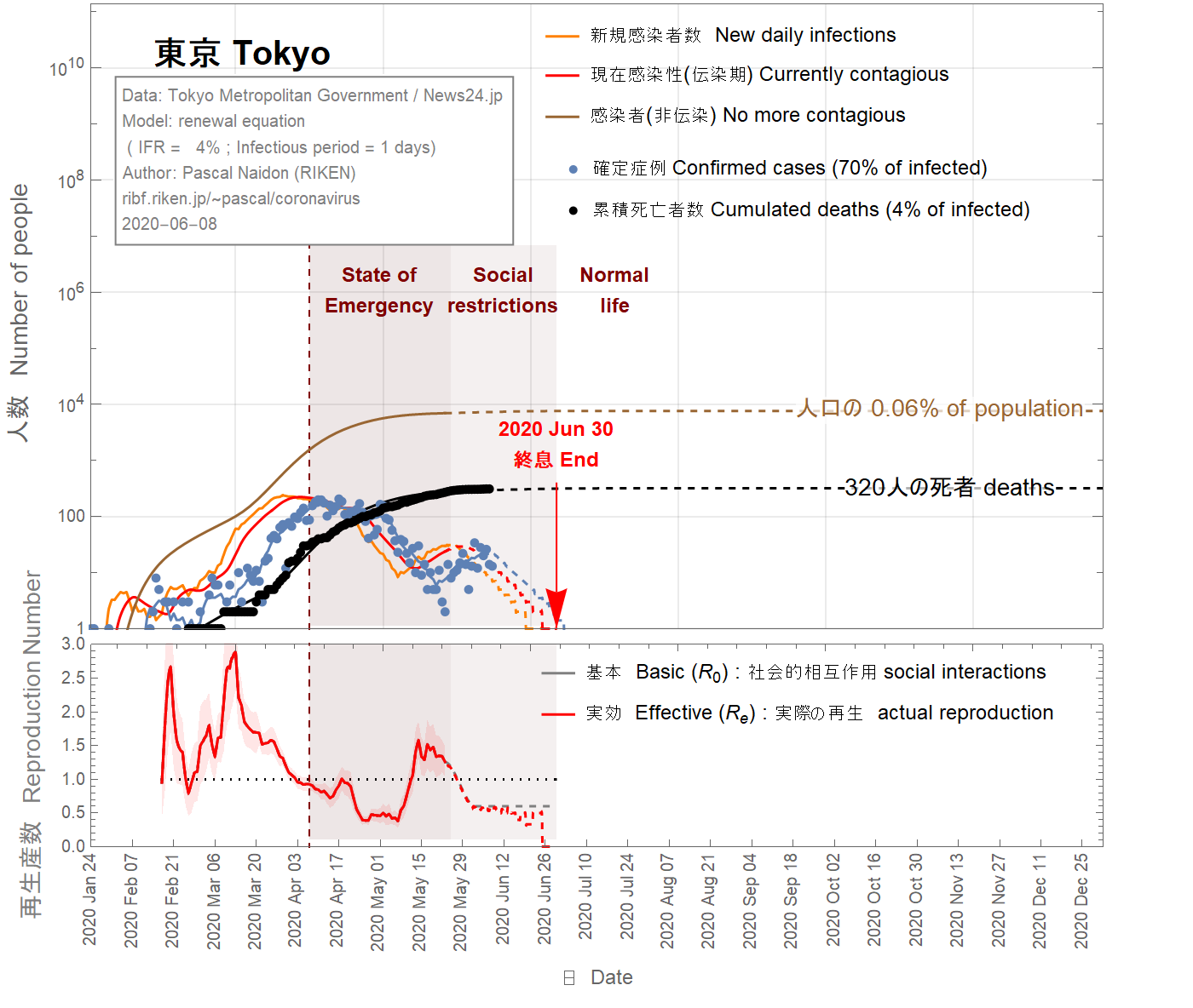
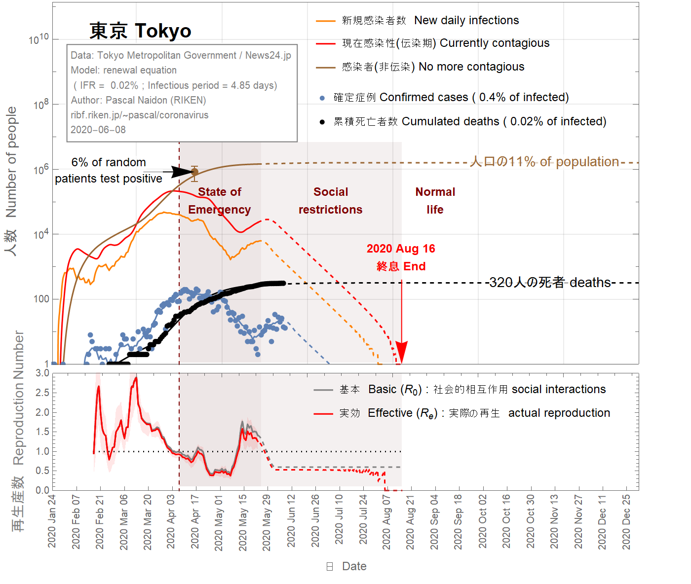
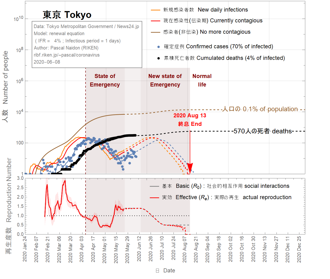
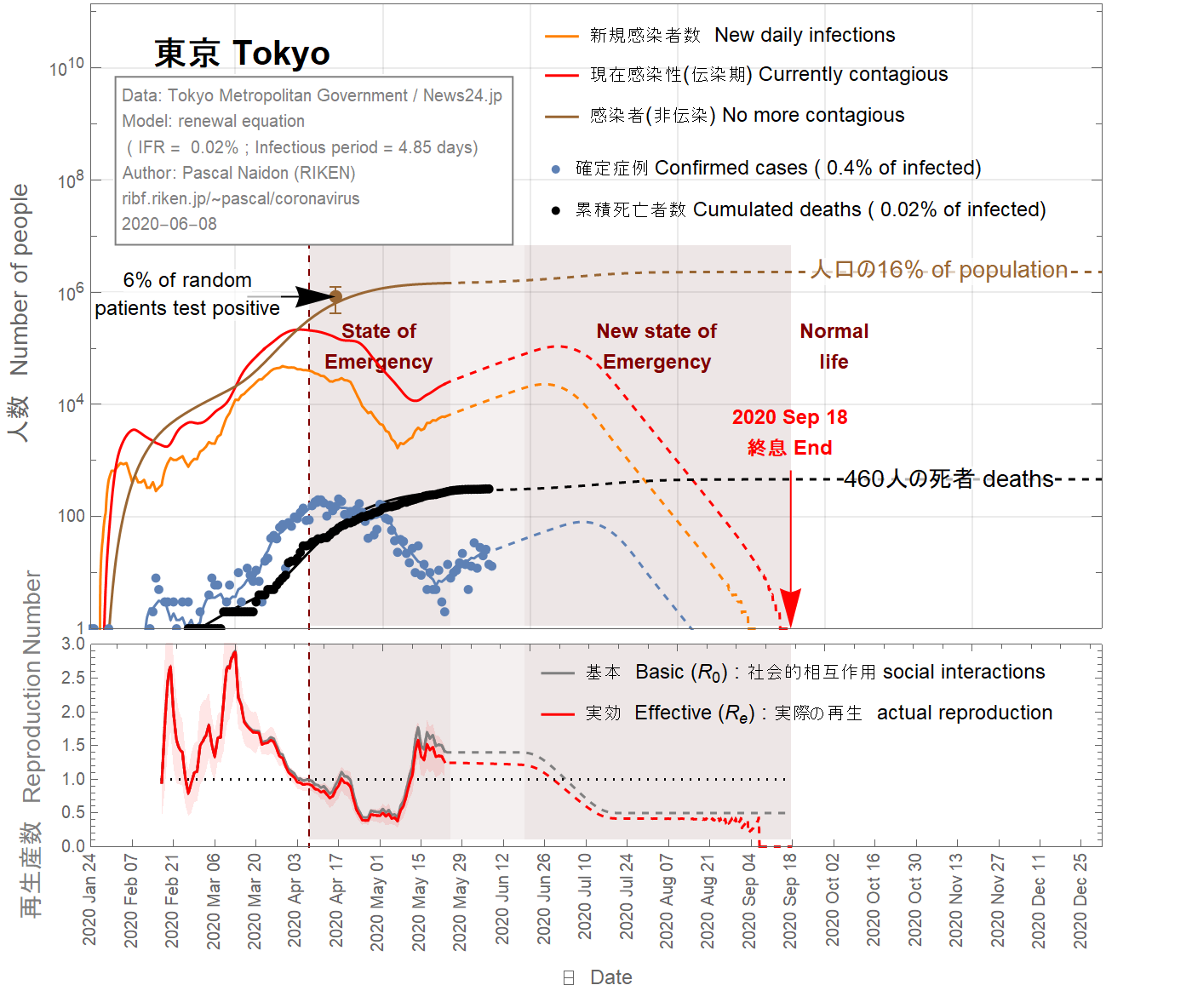
It is difficult to imagine that the infection fatality ratio (IFR) in Tokyo could be larger than the largest value for France (4%). Taking this value, one obtains (see Fig 7) that almost all real cases are confirmed, which is unlikely. On April 23rd 2020, it was reported that 4 of 67 patients admitted to Keio University Hospital for conditions unrelated to the coronavirus tested positive for the virus. This would indicate that between 3% and 9% of the population in Tokyo has been infected. To match this range, the IFR has be to be as small as 0.02% (see Fig 9), which would mean that as few as 0.4% of infected people are detected. This situation sounds also unlikely.
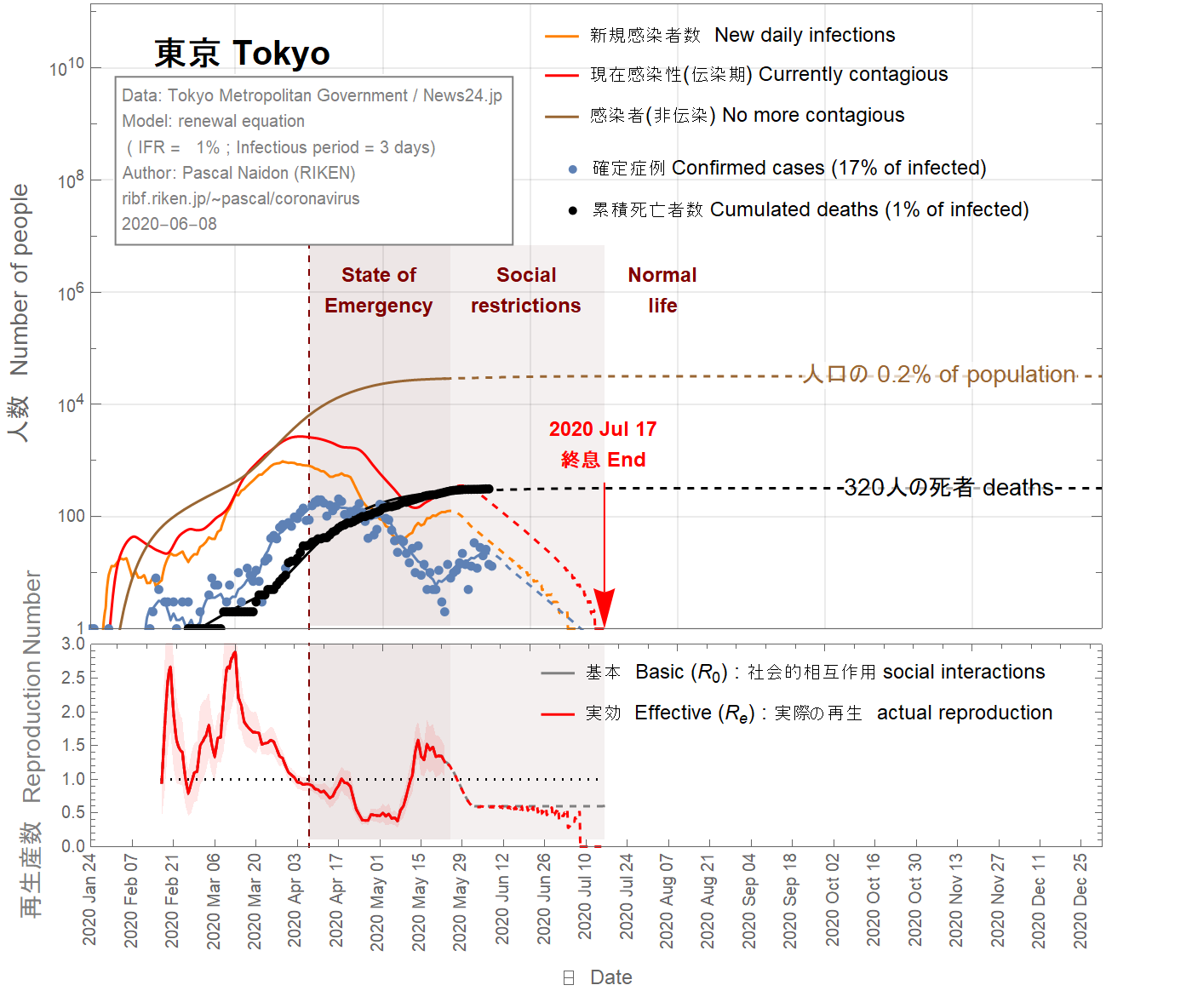
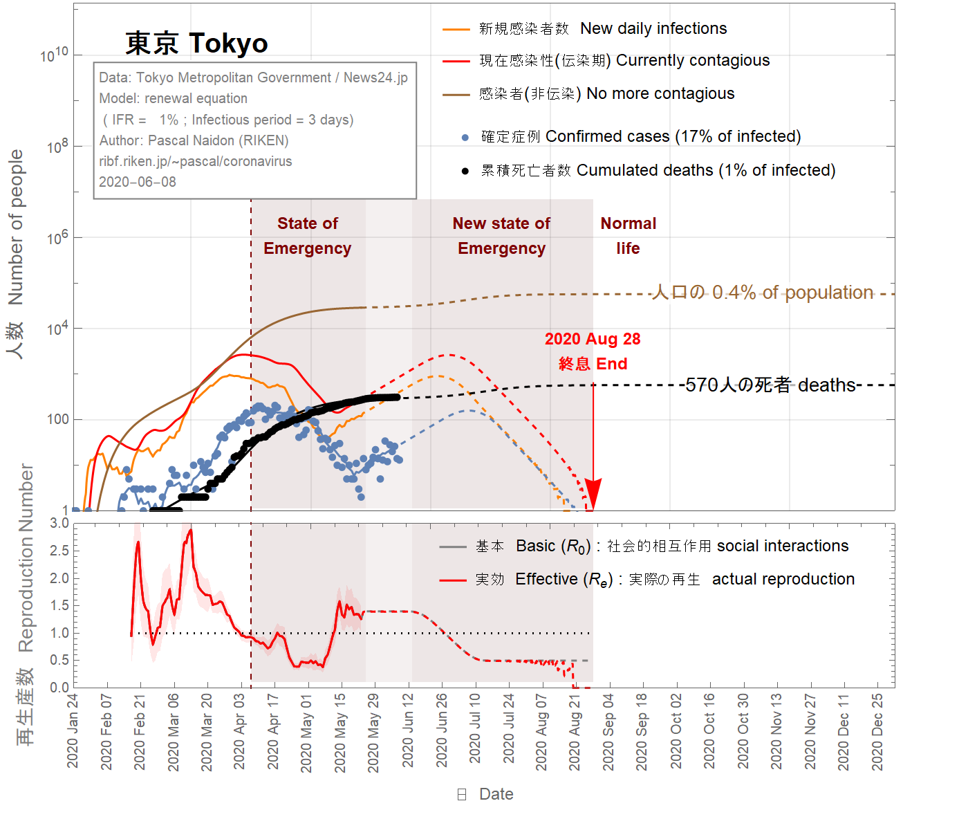
There is therefore a large uncertainty on the infection fatality ratio in Tokyo (from 4% to 0.02%). Figure 8 shows the results for an intermediate value of 1%. In this case, about 0.2% of the Tokyoite population would have been infected by now.
Il est difficile d'imaginer que le taux de mortalité par infection (IFR) à Tokyo puisse être supérieur à la valeur la plus élevée pour la France (4%). En prenant cette valeur, on obtient (voir figure 7) que presque tous les cas réels sont confirmés, ce qui est peu probable. Le 23 avril 2020, il a été rapporté que 4 des 67 patients admis à l'hôpital universitaire de Keio pour des conditions sans rapport avec le coronavirus ont été testés positifs au coronavirus. Cela indiquerait qu'entre 3% et 9% de la population de Tokyo a été infectée. Pour correspondre à cette plage, l'IFR doit être aussi petit que 0,02% (voir figure 9), ce qui signifie que seulement 0,4% des personnes infectées sont détectées. Cette situation semble également peu probable.
Il existe donc une grande incertitude sur le taux de mortalité par infection à Tokyo (de 4% à 0,02%). La figure 8 montre les résultats pour une valeur intermédiaire de 1%. Dans ce cas, environ 0,2% de la population tokyoïte aurait été infectée à ce jour.
東京の感染致死率(IFR)がフランスの最大値(4%)よりも大きいという可能性は、想像しにくいです。この値(4%)を使用すると、ほとんどすべての実際のケースが確認されていることがわかります(図7を参照)。 2020年4月23日、 67人の患者のうち4人が、コロナウイルスはウイルス陽性であした。これは、東京の人口の3%から9%が感染していることを示します。この範囲に一致させるには、IFRを0.02%(図9を参照)まで小さくする必要があります。これは、感染者のわずか0.4%が検出されることを意味します。この状況も起こりそうにありません。
したがって、東京の感染致死率には大きな不確実性があります(4%から0.02%)。図8は、中間値1%の結果を示しています。この場合、東京人の人口の約0.2%がこれまでに感染していたということになります。
End of epidemic
The situation in Tokyo has become problematic in the last few days. Although it appeared that the daily number of confirmed cases would reach zero by the beginning of June, recent numbers seem to indicate a return of infections (which would have started two weeks ago, due to confirmation delays), and a basic reproduction number going back to values larger than 1. In this situation, it is extremely difficult to make any projection.
This situation could be due to a local cluster that could be tracked and isolated, in which case the daily number of confirmed cases would quickly vanish within June 2020, as illustrated in Fig 7, 8, 9.
This could also be the start of a second wave. This is illustrated in Fig 10, 11, 12. Since the state of emergency has been lifted on May 25th and there is a current trend towards going back to normal life, one can assume that the basic reproduction number goes back to a value of 1.3, comparable with its value before the state of emergency. The daily number of confirmed cases would then keep increasing. As a result, it is assumed that state of emergency would be reinstated around June 10th, gradually reducing the basic reproduction number down to 0.5 over one month. In this scenario, about 100 extra deaths could result from the second wave, and the epidemic would be extended to August 2020.
Fin de l'épidémie
La situation à Tokyo est devenue problématique ces derniers jours. Bien qu'il semble que le nombre quotidien de cas confirmés devait atteindre zéro au début de juin, les chiffres récents semblent indiquer un retour des infections (qui se serait donc passé il y a deux semaines, compte-tenu des délais) et un nombre de reproduction de base revenant à des valeurs supérieures à 1. Dans cette situation, il est extrêmement difficile de faire une projection.
Cette situation pourrait être due à un foyer d'infection localisé qui serait rapidement détecté et maîtrisé, auquel cas le nombre quotidien de cas confirmés pourrait rapidement disparaître en juin 2020, comme l'illustrent les figures 7, 8, 9.
Cela pourrait également être le début d'une deuxième vague . Ceci est illustré sur les figures 10, 11, 12. Étant donné que l'état d'urgence a été levé le 25 mai et qu'il existe une tendance actuelle à revenir à la vie normale, on peut faire l'hypothèse que le nombre de reproduction de base va revenir durablement à une valeur de 1,3, comparable à sa valeur avant l'état d'urgence. Le nombre quotidien de cas confirmés continuerait alors d'augmenter. En conséquence, il est supposé que l'état d'urgence serait rétabli vers le 10 juin, réduisant progressivement le nombre de reproduction de base à 0,5 sur un mois. Dans ce scénario, environ 100 décès supplémentaires pourraient résulter de la deuxième vague, et l'épidémie serait prolongée jusqu'en août 2020.
流行の終息
ここ数日、東京の状況は問題になっています。 6月の初めまでに1日あたりの確認症例数はゼロになると思われますが、最近の数値は感染の再発を示しているようです(確認の遅れにより、2週間前から始まっていたのでしょう)。この状況では、予測を行うことは非常に困難です。
この状況は、追跡隔離可能なローカルクラスターが原因である可能性があります。この場合、図7、8、9に示すように、確認された症例の1日あたりの数は、2020年6月以内に急速に減っていきます。
これは、第二波の始まりでもあります。これを図10、11、12に示します。緊急事態が5月25日に解除され、現在の通常の生活に戻る傾向があるため、基本再生産数は緊急事態以前の値と同等である1.3に戻ると想定されます。その後、確認された症例の毎日の数は増加し続けます。その結果、6月10日頃に緊急事態が復活し、1か月間で基本再生産数が0.5まで徐々に減少すると想定されます。このシナリオでは、第2波によって約100人の追加の死亡が発生する可能性があり、流行は2020年8月まで延びます。
Data source
Sources
情報源
:
Confirmed cases
Cas confirmés
感染者
: Tokyo Metropolitan Government stopcovid19
Reported deaths
Décès
死亡者数:
News24.jp
Random patient tests
Tests de patients aléatoires
ランダムな患者テスト:
NHK
Saitama prefecture
Région de Saitama
埼玉県
Applying the same analysis to the prefecture of Saitama, I obtain the following results.
En appliquant la même analyse à la préfecture de Saitama, j'obtiens les résultats suivants.
埼玉県にも同様の分析を適用すると、次のような結果が得られます。
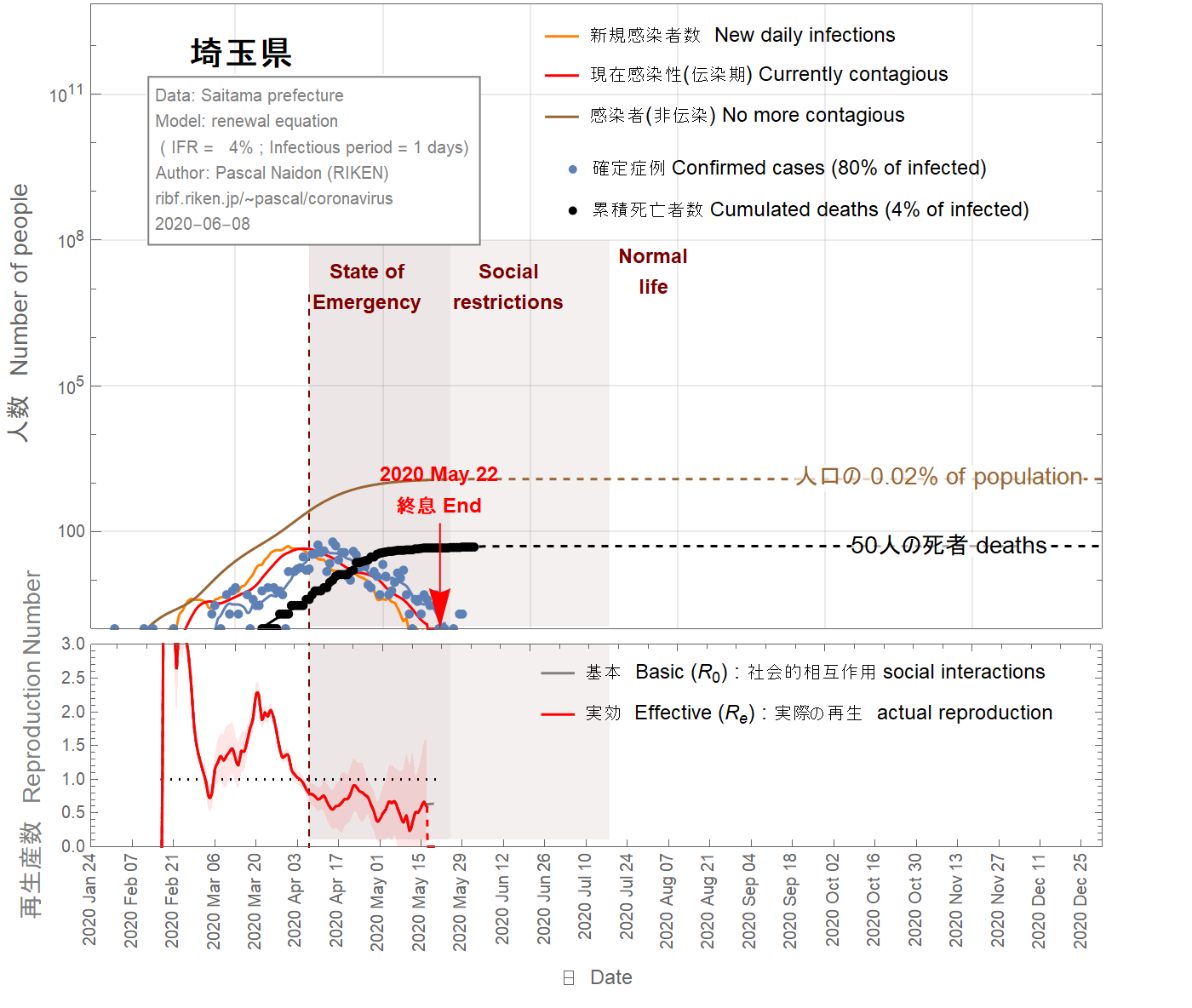
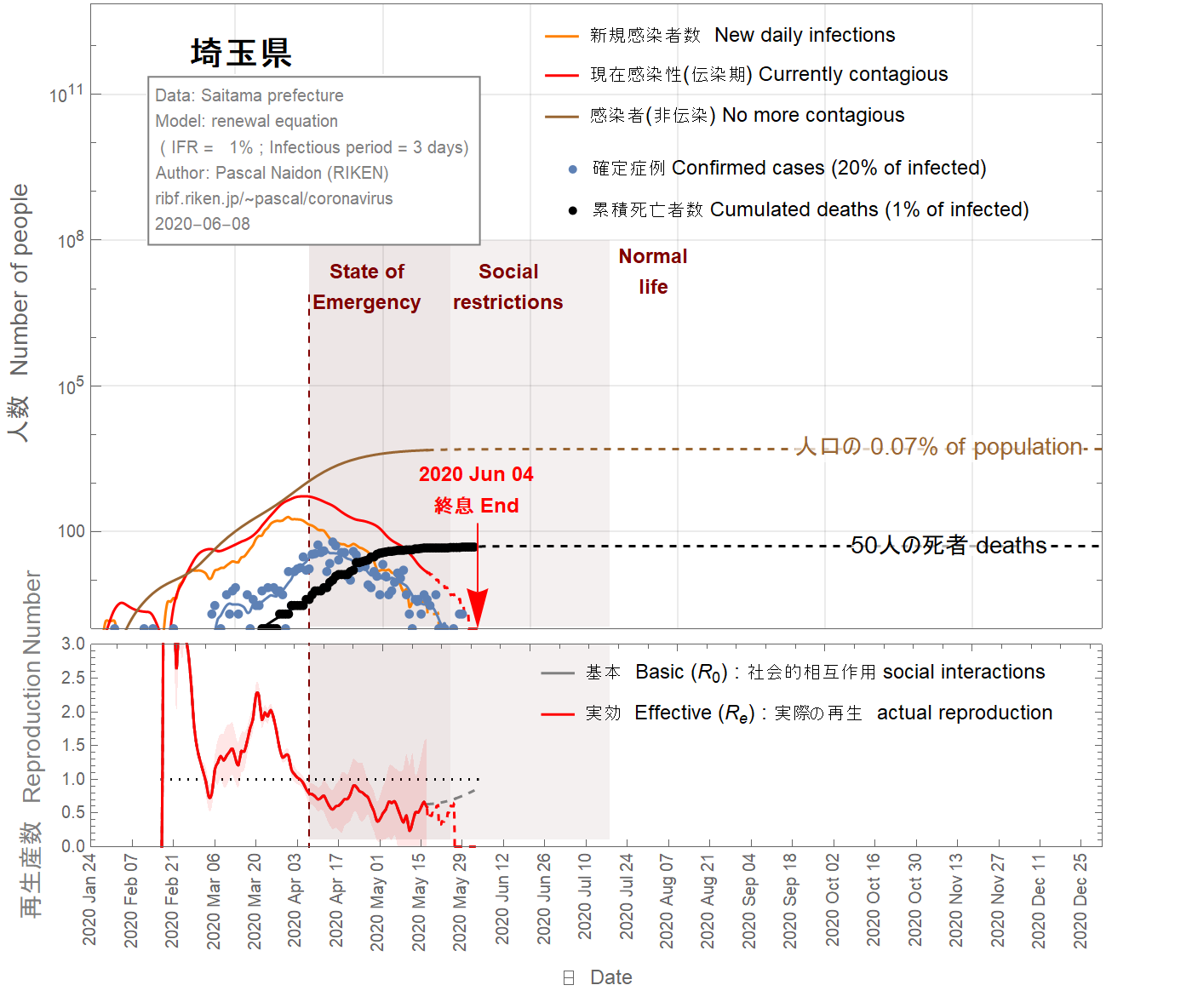
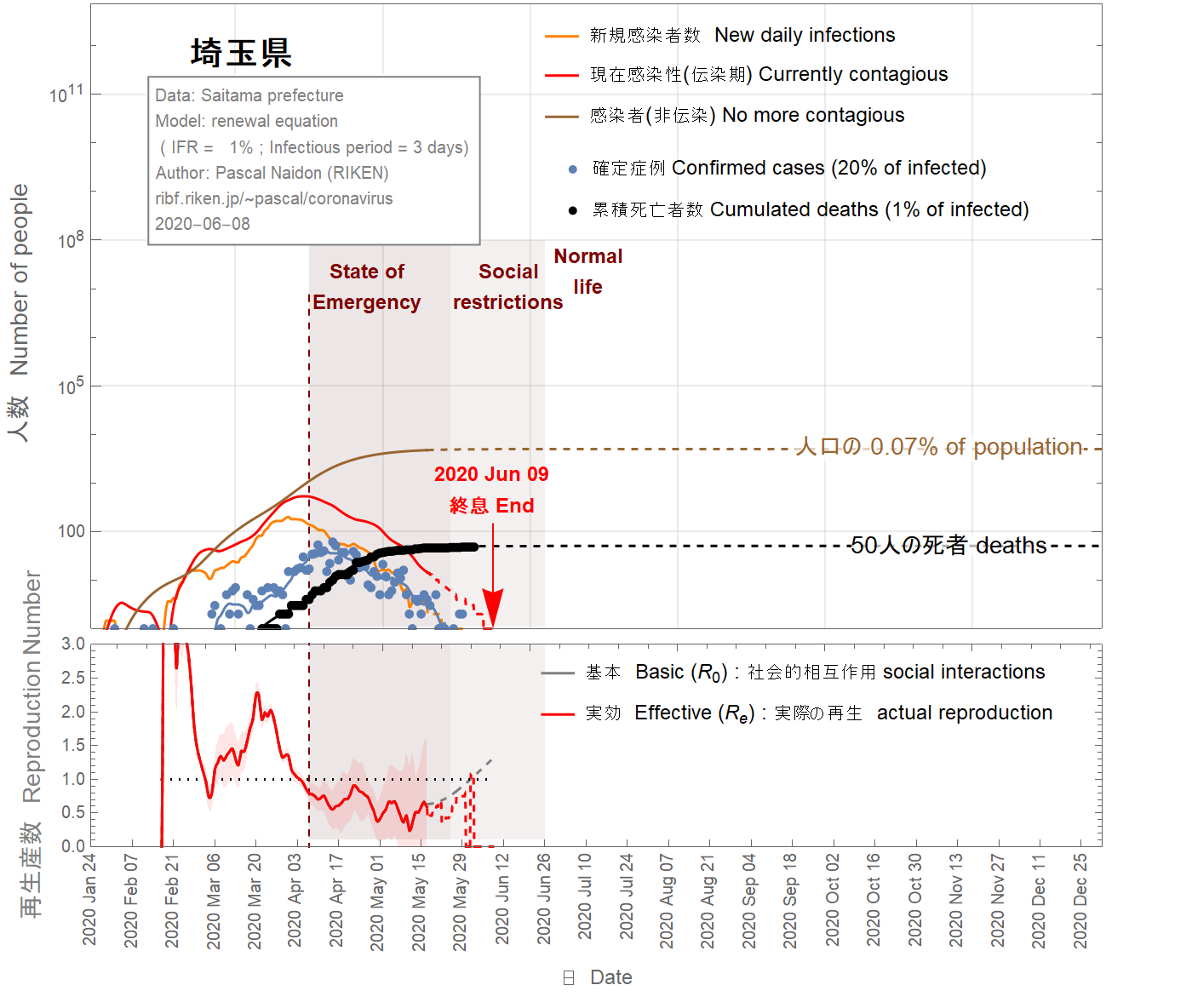
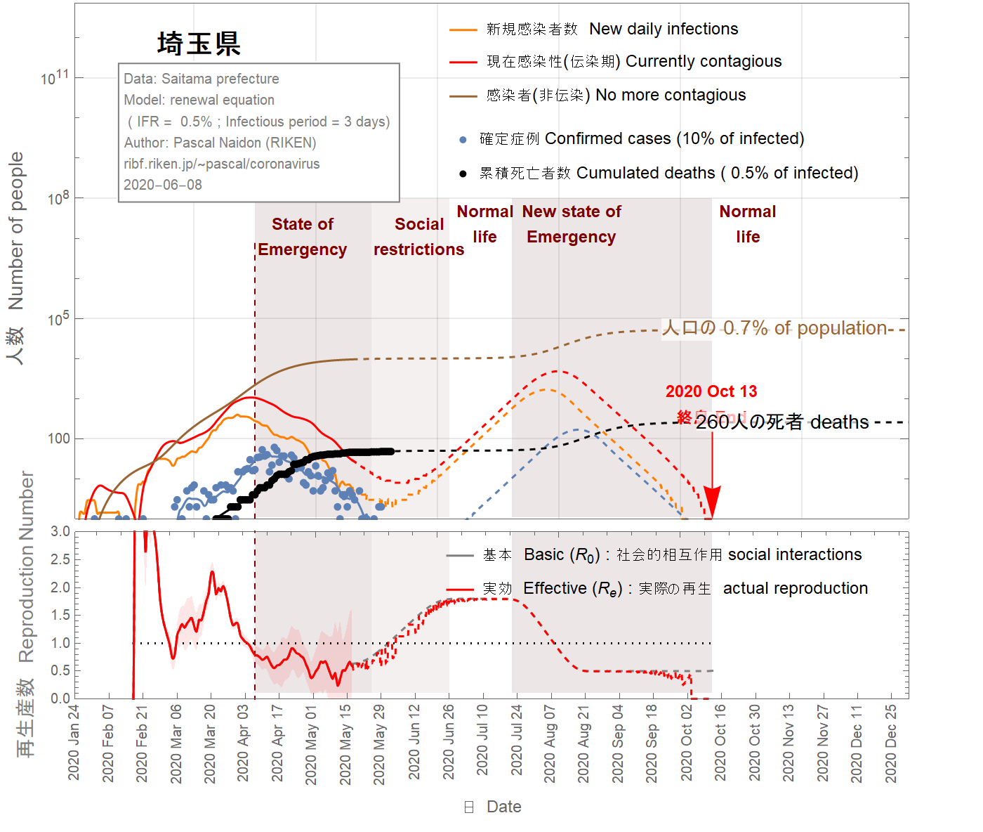
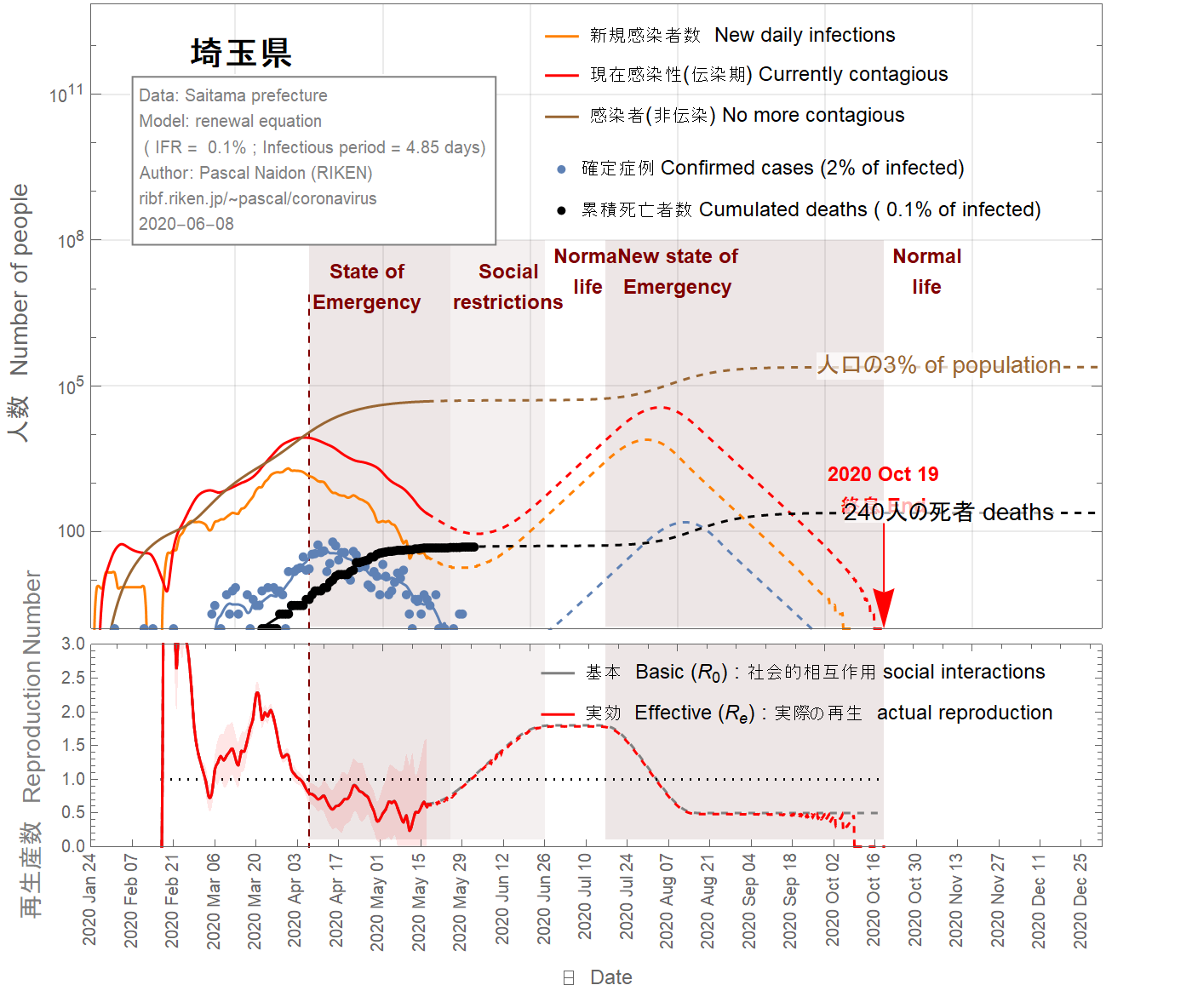
End of epidemic
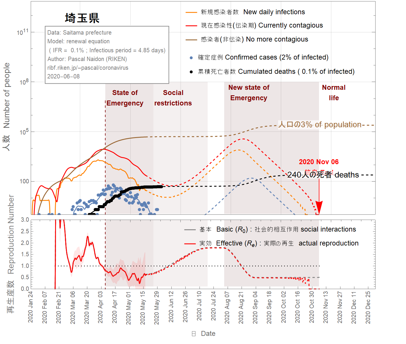
The situation in the Saitama prefecture looks well under control with an imminent end of the epidemic, as shown in Figs 13-16. Nevertheless, because of the two-week delay between confirmed cases and the actual infections, it is too soon to exclude the possibility of second wave. In the figures 13-16, I assumed that return to normal life gradually started on May 17 such that the basic reproduction number reaches two months later the value of 1.8. As one can see, a second wave is relatively unlikely unless the infection fatality ratio is smaller than 0.5%. However, a faster return to normal life (in 40 days) increases the chance of second wave, as shown in the figures 17-19. Moreover, the possible influx of infectors coming from other areas (like nearby Tokyo) have not been taken into account and may increase the probability of a second wave.
Fin de l'épidémie
La situation dans la préfecture de Saitama semble bien maîtrisée avec une fin imminente de l'épidémie, comme le montrent les figures 13-16. Néanmoins, en raison du délai de deux semaines entre les cas confirmés et les infections réelles, il est trop tôt pour exclure la possibilité d'une deuxième vague. Dans les figures 13-16, on a fait l'hypothèse que le retour à la vie normale a commencé progressivement le 17 mai de sorte que le nombre de reproduction de base atteint deux mois plus tard la valeur de 1.8. Comme on peut le voir, une deuxième vague est relativement peu probable à moins que le taux de mortalité par infection ne soit inférieur à 0,5%. Cependant, un retour plus rapide à la vie normale (en 40 jours) augmente les chances de deuxième vague, comme le montrent les figures 17-19. De plus, l'afflux possible d'infecteurs provenant d'autres régions (telles que Tokyo) n'a pas été pris en compte et peut augmenter la probabilité d'une deuxième vague.
流行の終息
埼玉県の状況は、図13-16に示すように、まもなく流行が終息し、制御できる状況になるように見えます。 それにもかかわらず、確定した症例と実際の感染との間には2週間の遅延があるため、第二波の可能性を排除するには早すぎます。次の図では、5月17日から徐々に通常の生活に戻り、基本再生産数が2か月後に1.8に達したと仮定しています。 ご覧のとおり、感染の致死率が0.5%未満でない限り、第二波の可能性は、比較的低いでしょう。 ただし、図17-19に示すように、通常の生活への復帰が早い(40日で)場合、第二波の可能性が高くなります。また、他の地域(東京の近くなど)からの感染の可能性は考慮されておらず、第二波の可能性が高くなり得ます。
Data source
Sources
情報源
:
Confirmed cases
Cas confirmés
感染者
: Saitama prefecture
Reported deaths
Décès
死亡者数:
Saitama prefecture
Although these simple calculations cannot be taken as realistic projections of the epidemic, they give us some idea of possible outcomes in the coming months or year. An important source of uncertainty is the infection fatality ratio, as well as the impossibility to predict the basic reproduction number, which reflects government and social reactions.
Bien que ces calculs simples ne puissent pas être considérés comme des projections réalistes de l'épidémie, ils nous donnent une idée des résultats possibles dans les mois ou l'année à venir. Une source importante d'incertitude est le taux de mortalité par infection, ainsi que l'impossibilité de prédire le nombre de reproduction de base, qui reflète les réactions gouvernementales et sociales.
これらの単純な計算は、流行の現実的な予測と見なすことはできませんが、今後数か月または1年で起こり得る結果についての示唆を与えてくれます。不確実性の主たる要因は、感染の致死率、および政府と社会の反応を反映する基本再生算数を予測することが不可能であることです。


 riken.jp